Plane Curve Book

The book is now out in Kindle, paperback and notebook formats from Wolfram Media. Go to wolfr.am/DaytonCurves for current information and links. The link to Amazon will allow you (look inside) to read the first section which gives an idea of my methodology.

In addition there is a free summary of the book in Wolfram's The Mathematica Journal.

This article is also available in notebook (.nb) and Wolfram Reader (.cdf) format. The global functions used in this article are available in Mathematica notebook form. These can be executed in Mathematica. If you do not have access to Mathematica and just want to look at the full code you can read this notebook using the free Wolfram CDF player.

For those readers of the TMJ article who might want to get more information on a particular chapter individual chapter notebooks and additional material are available for download at Chapter Notebooks and More. If you want more than a few a better option is to to the Wolfram media link above and download the zip file. You do need to download the Appendix 2, Global Functions (.nb 1.1MB) notebook and Evaluate initialization cells before using any of the other notebooks.

For the convenience of all users of the software defined in this book we have an index to Global Functions (PDF) which lists all the Global Functions (Appendix 2) alphabetically, giving syntax and location, by section, where further information on this function can be found in the book, chapter notebooks or Global Function notebook.

One challenge in production of this book is that both the typesetting an execution of code is done by Mathematica at the same time. For technical reasons some code did not execute properly when the the fixed print versions were typeset. The notebook versions in Chapter Notebooks have been, or soon will be, updated where necessary to fix these errors.

• Section 1.6 page 16 (Make sure for In[46] the cell property "evaluatable" is set.)
  In[46]    gs = sqFree[g, x, y, 1.*^-12]
Out[46]   0.132808 x - 0.132808 x^3 - 0.132808 y + 0.132808 x^2 y - 0.132808 x y^2 + 0.132808 y^3

  In[48]    gs = Expand[gs/Coefficient[gs, x^3]]
Out[48]   -1. x + 1. x^3 + 1. y - 1. x^2 y + 1. x y^2 - 1. y^3

• Section 2.4, page 35 The total degree tDeg function is defined incorrectly here. It is not used later in Chapter 2 but the correct version in the Global Functions Appendix and notebook should be used later, eg. in Chapter 5.
• Section 3.2, page 45 (computer error)
  In[18]    run2 = tangentRealPoints[f, k, x, y]
Out[18]   {{1.15237, 1.27611}, {0.707107, 0.5}, {0.707107, 0.5}, {0., -0.5}, {0., -0.5}, {0.928493, -0.857753}, {-0.754479, 0.417765}, {-0.707107, 0.5}, {-0.707107, 0.5}}

• Section 3.4, page 50 (failure to update from earlier version)
  In[50]    fbow = x^4 - x^2 y + y^3;
          fmin = -x^2 y + y^3;
          infiniteRealPoints[fmin, x, y]
Out[50]   {{-5.22164, -5.22164, 0}, {-4.1098, 0., 0}, {-3.38833, 3.38833, 0}}

• Section 3.5,page 53 (failure to update)
  In[69]    fm1 = Factor[pointMinForm[f, {-2, 0}, x, y]]
Out[69]   16 (x - y) (x + y)

  In[71]    fm2 = Factor[pointMinForm[f, {2, 0}, x, y]]
Out[71]   16 (x - y) (x + y)

• Section 5.3, pages 98-99 (Make sure dTol = 1.*^-12)
  In[22]    intersectionMultiplicity[y - x^2 + 1, y^2 - x^2 - 5, {2, 3}, dTol]
  Out[22]   1

  In[23]    intersectionMultiplicity[y + 1/3 x^2 - 2 x - 1/3, y^2 - x^2 - 5, {2, 3}, dTol]
  Out[23]   2

  In[24]    intersectionMultiplicity[y - x^3, y, {0, 0}, dTol]
  Out[24]   3

  In[26]    intersectionMultiplicity[y - x - x^3, y - x - y^3, {0, 0}, dTol]
  Out[26]   5

  In[27]    intersectionMultiplicity[y^2 - x^3, y - 3 x, {0, 0}, dTol]
  Out[27]   2

  In[28]    intersectionMultiplicity[x^2 + y^2, y - 3 x, {0, 0}, dTol]
Out[28]   2

• Section 5.4 p 106 The singularity Theorem. This has been redone, see the Wolfram Community post The Number of Singular Points on an algebraic curve

• Chapter 6 The main function FLT requires the function homog not defined in this chapter. Be sure to run Global Functions before executing the notebook version of this chapter.

• Section 7.2 p.147. Paragraph is garbled, a better version is

• Section 7.3, p. 157 (Trigonometric Parameterization) The code for P2C in the second line does not execute. Click "Execute" on menu Cell,"cell properties".
NEW 2021 A function ncr2[S] has been added which takes 5 points in general position directly to a rational parameterization.
• Section 7.6, p.167 (Failure to update from earlier version)
  In[165]   {intersectionMultiplicity[y^2 - x^3 - x^2, l, {0, 0}, dTol],
          intersectionMultiplicity[y^2 - x^3, l, {0, 0}, dTol],
          intersectionMultiplicity[(y - x^2) (y + x^4), l, {0, 0}, dTol],
          intersectionMultiplicity[x y (x - y), l, {0, 0}, dTol]}
Out[165]  {2, 2, 2, 3}

  On page 168 in the second paragraph the formula for gt is wrong, it should be gt = g1 + t g2. Note that at the bottom of p. 169 the correct formula was used.

  Below this on p. 168 the variable d was assumed non-initialized but apparently was. The correction is
  In[166]  Clear[d]
         Expand[(d-1)(d-2)/2+2d-3]
Out[166] -2+d/2+d^2/2

  On page 168 we have the same problem. Hopefully now d is unevaluated so
  In[167]   Expand[2((d-1)(d-2)/2)+2d-3]
Out[167] -1-d+d^2
  But this is d(d-1)-1.

  In Mathematica 11.3 there was a bug in built-in function Resultant so on page 171 we used the work-around SetPrecision[g[t],20] . This bug has been fixed in Mathematica 12 so g[t] is sufficient.

• Section 8.3, p.188 In the example of a rational function the line for L4 gives an error message when executing the notebook version. The reason is pathFinderT begins with a capital P instead of the correct small p. However the printed and notebook versions have the correct graphics.
• Section 8.5 p.194-195 The graphic for Example 3 was omitted. It does appear on p. 206. For original notebook version this is also a problem, the picture is in Section 8.7.

• Section 8.7 p. 204 Example A2 The graphic for Example A2, affine hyperbola, is wrong, the correct picture was shown on p 194. This can be corrected in the notebook version by changing the first line of in[169] to

            Hp = Table[{Sqrt[y^2 + 4], y}, {y, -6, 6, .201}]

  This avoids hitting the x-axis which is ambiguous.

• Section 9.1, p.213 The proof of Harnack's theorem is garbled. This has been fixed in the notebook version on this website, for the convience of those with fixed print copies here is a PDF version of the corrected proof as well the other chapter 9 issues below.
• Section 9.2 The argument to dDiagram is an association with keys ordered pairs {a,b} and values 0,1. For diagrams of dimension d each ordered pair with |a|+|b| ≤ d must appear as a key otherwise there was a horrible error message. To avoid this message this function now checks that this condition holds and aborts if it does not hold. Also in the A2-Global Functions notebook on this website there is a new function gaussDiagram for use on sparse polynomials since viroDiagram does not work.
• Notebook versions Chapters 9,10, Global Functions. There are 6 graphics primitives given to label the infinite points in DDiagrams, labelI,...,label24. These are coded in 9.6 the Appendix to Chapter 9, page 258 in the printed book, and also in A2-Global Functions. These primitives do not work in Mathematica 12 giving execution errors in the notebooks throughout Chapters 9,10,A2. Actually they were not well coded originally and are not actually needed, they can be given by the symbolic graphics function Text as easily as using these primitives. As an example the example in A2 for section 9.2 should be

  
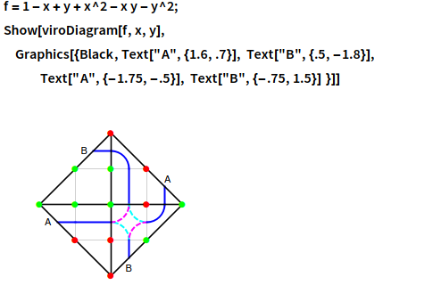
  Note here that the coordinates in DDiagrams are such that the dots are given by integer points with the center (origin) at {0,0}. It may some trial and error to get the coordinates right. The notebooks for 9,10 and A2 in Chapter Notebooks have been updated to reflect this usage.

• Section 9.3, p. 242 The diamond diagram is incompletely labeled. See Correction to Chapter 9
  
  

  Let me know at barry@barryhdayton.us if you find other places where there is a problem.